前言🔖
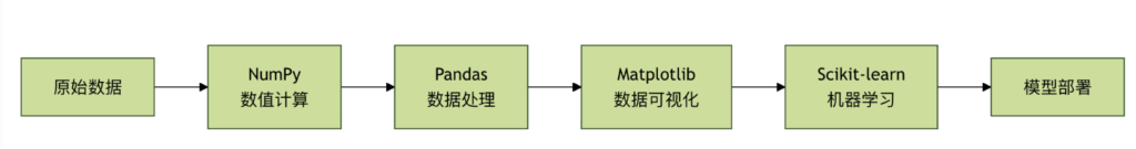
本章将为你详细介绍机器学习中最核心的四个 Python 库:NumPy、Pandas、Matplotlib 和 Scikit-learn。
机器学习库就像一套专业的工具箱,每个库都有特定的用途,配合使用可以完成复杂的机器学习任务。
四大核心库的角色
- Numpy:数值计算的基础,提供高效的数组操作
- Pandas:数据处理的利器,提供数据结构和分析工具
- Matplotlib:数据可视化的画笔,创建各种图表
- scikit-learn:机器学习的瑞士军刀,提供完整的 ML 工具链
NumPy:数值计算的基础🔖
什么是 NumPy?
NumPy 就像是数学计算的计算器,但功能强大无数倍。它是 Python 科学计算的基础库,提供了高效的多维数组对象。
NumPy 的核心概念
🔹1. 数组(Array)
# NumPy 数组基础操作
import numpy as np

# 创建数组的不同方式
print("=== NumPy 数组创建 ===")

# 从列表创建
arr1 = np.array([1, 2, 3, 4, 5])
print(f"从列表创建:{arr1}")

# 创建等差数组
arr2 = np.arange(0, 10, 2)  # 0到10,步长为2
print(f"等差数组:{arr2}")

# 创建等间隔数组
arr3 = np.linspace(0, 1, 5)  # 0到1,5个点
print(f"等间隔数组:{arr3}")

# 创建特殊数组
zeros_arr = np.zeros((2, 3))  # 2行3列的零数组
ones_arr = np.ones((2, 3))    # 2行3列的一数组
identity_arr = np.eye(3)      # 3x3单位矩阵

print(f"零数组:\n{zeros_arr}")
print(f"一数组:\n{ones_arr}")
print(f"单位矩阵:\n{identity_arr}")
=== NumPy 数组创建 ===
从列表创建:[1 2 3 4 5]
等差数组:[0 2 4 6 8]
等间隔数组:[0.   0.25 0.5  0.75 1.  ]
零数组:
[[0. 0. 0.]
 [0. 0. 0.]]
一数组:
[[1. 1. 1.]
 [1. 1. 1.]]
单位矩阵:
[[1. 0. 0.]
 [0. 1. 0.]
 [0. 0. 1.]]
🔹2. 数组操作
# 数组的基本操作
print("\n=== 数组基本操作 ===")

# 数组属性
arr = np.array([[1, 2, 3], [4, 5, 6]])
print(f"数组:\n{arr}")
print(f"形状:{arr.shape}")
print(f"维度:{arr.ndim}")
print(f"元素个数:{arr.size}")
print(f"数据类型:{arr.dtype}")

# 数组索引和切片
print(f"第一行:{arr[0]}")
print(f"第一列:{arr[:, 0]}")
print(f"元素[1,2]:{arr[1, 2]}")

# 数组运算
arr1 = np.array([1, 2, 3])
arr2 = np.array([4, 5, 6])

print(f"加法:{arr1 + arr2}")
print(f"乘法:{arr1 * arr2}")
print(f"点积:{np.dot(arr1, arr2)}")

# 统计函数
data = np.array([1, 2, 3, 4, 5, 6, 7, 8, 9, 10])
print(f"均值:{np.mean(data)}")
print(f"标准差:{np.std(data)}")
print(f"最大值:{np.max(data)}")
print(f"最小值:{np.min(data)}")
print(f"中位数:{np.median(data)}")
=== 数组基本操作 ===
数组:
[[1 2 3]
 [4 5 6]]
形状:(2, 3)
维度:2
元素个数:6
数据类型:int64
第一行:[1 2 3]
第一列:[1 4]
元素[1,2]:6
加法:[5 7 9]
乘法:[ 4 10 18]
点积:32
均值:5.5
标准差:2.8722813232690143
最大值:10
最小值:1
中位数:5.5
🔹3.NumPy 实际应用示例
# NumPy 实际应用:简单线性回归
def numpy_linear_regression():
    """使用 NumPy 实现简单线性回归"""

    # 生成示例数据
    np.random.seed(42)
    X = 2 * np.random.rand(100, 1)  # 特征
    y = 4 + 3 * X + np.random.randn(100, 1)  # 标签 + 噪声

    # 添加 x0 = 1 到 X
    X_b = np.c_[np.ones((100, 1)), X]  # 添加偏置项

    # 使用正规方程求解:θ = (X^T * X)^(-1) * X^T * y
    theta_best = np.linalg.inv(X_b.T.dot(X_b)).dot(X_b.T).dot(y)

    print("=== NumPy 线性回归示例 ===")
    print(f"学习到的参数:截距={theta_best[0][0]:.2f}, 斜率={theta_best[1][0]:.2f}")

    # 预测
    X_new = np.array([[0], [2]])
    X_new_b = np.c_[np.ones((2, 1)), X_new]
    y_predict = X_new_b.dot(theta_best)

    print(f"预测结果:X=0 时 y={y_predict[0][0]:.2f}, X=2 时 y={y_predict[1][0]:.2f}")

    return theta_best, X, y

# 运行示例
theta, X, y = numpy_linear_regression()
=== NumPy 线性回归示例 ===
学习到的参数:截距=4.22, 斜率=2.77
预测结果:X=0 时 y=4.22, X=2 时 y=9.76
Pandas:数据处理的利器🔖
什么是 Pandas?
Pandas 就像是数据处理的瑞士军刀,提供了强大的数据结构和数据分析工具,特别适合处理表格型数据。
Pandas 的核心数据结构
🔹1. Series(一维数据)
# Pandas Series 基础操作
import pandas as pd

print("=== Pandas Series ===")

# 从列表创建 Series
s1 = pd.Series([1, 2, 3, 4, 5])
print(f"从列表创建:\n{s1}")

# 带索引的 Series
s2 = pd.Series([10, 20, 30], index=['a', 'b', 'c'])
print(f"\n带索引的 Series:\n{s2}")

# 从字典创建 Series
s3 = pd.Series({'数学': 90, '英语': 85, '物理': 88})
print(f"\n从字典创建:\n{s3}")

# Series 操作
print(f"\n访问元素:s2['b'] = {s2['b']}")
print(f"切片:s2[0:2] =\n{s2[0:2]}")
print(f"统计信息:\n{s2.describe()}")
=== Pandas Series ===
从列表创建:
0    1
1    2
2    3
3    4
4    5
dtype: int64

带索引的 Series:
a    10
b    20
c    30
dtype: int64

从字典创建:
数学    90
英语    85
物理    88
dtype: int64

访问元素:s2['b'] = 20
切片:s2[0:2] =
a    10
b    20
dtype: int64
统计信息:
count     3.0
mean     20.0
std      10.0
min      10.0
25%      15.0
50%      20.0
75%      25.0
max      30.0
dtype: float64
🔹2. DataFrame(二维数据)
# Pandas DataFrame 基础操作
print("\n=== Pandas DataFrame ===")

# 创建 DataFrame
data = {
    '姓名': ['张三', '李四', '王五', '赵六'],
    '年龄': [25, 30, 35, 28],
    '城市': ['北京', '上海', '广州', '深圳'],
    '薪资': [15000, 20000, 18000, 22000]
}

df = pd.DataFrame(data)
print("原始 DataFrame:")
print(df)

# DataFrame 基本操作
print(f"\nDataFrame 形状:{df.shape}")
print(f"\n列名:{list(df.columns)}")
print(f"\n数据类型:\n{df.dtypes}")

# 选择数据
print(f"\n选择'姓名'列:\n{df['姓名']}")
print(f"\n选择前两行:\n{df.head(2)}")
print(f"\n选择年龄大于28的行:\n{df[df['年龄'] > 28]}")

# 统计信息
print(f"\n数值列的统计信息:\n{df.describe()}")

# 添加新列
df['年薪'] = df['薪资'] * 12
print(f"\n添加年薪列后:\n{df}")
=== Pandas DataFrame ===
原始 DataFrame:
   姓名  年龄  城市     薪资
0  张三  25  北京  15000
1  李四  30  上海  20000
2  王五  35  广州  18000
3  赵六  28  深圳  22000

DataFrame 形状:(4, 4)

列名:['姓名', '年龄', '城市', '薪资']

数据类型:
姓名    object
年龄     int64
城市    object
薪资     int64
dtype: object

选择'姓名'列:
0    张三
1    李四
2    王五
3    赵六
Name: 姓名, dtype: object

选择前两行:
   姓名  年龄  城市     薪资
0  张三  25  北京  15000
1  李四  30  上海  20000

选择年龄大于28的行:
   姓名  年龄  城市     薪资
1  李四  30  上海  20000
2  王五  35  广州  18000

数值列的统计信息:
              年龄            薪资
count   4.000000      4.000000
mean   29.500000  18750.000000
std     4.203173   2986.078811
min    25.000000  15000.000000
25%    27.250000  17250.000000
50%    29.000000  19000.000000
75%    31.250000  20500.000000
max    35.000000  22000.000000

添加年薪列后:
   姓名  年龄  城市     薪资      年薪
0  张三  25  北京  15000  180000
1  李四  30  上海  20000  240000
2  王五  35  广州  18000  216000
3  赵六  28  深圳  22000  264000
🔹3. Pandas 数据处理示例
# Pandas 数据处理完整示例
def pandas_data_processing():
    """演示 Pandas 数据处理的完整流程"""

    print("=== Pandas 数据处理示例 ===")

    # 1. 创建示例数据
    np.random.seed(42)
    n_samples = 1000

    data = {
        '学生ID': range(1, n_samples + 1),
        '姓名': [f'学生{i}' for i in range(1, n_samples + 1)],
        '年龄': np.random.randint(18, 25, n_samples),
        '性别': np.random.choice(['男', '女'], n_samples),
        '数学成绩': np.random.normal(75, 15, n_samples),
        '英语成绩': np.random.normal(80, 12, n_samples),
        '物理成绩': np.random.normal(72, 18, n_samples),
        '班级': np.random.choice(['一班', '二班', '三班'], n_samples)
    }

    df = pd.DataFrame(data)

    # 2. 数据清洗
    print("原始数据形状:", df.shape)

    # 处理异常值(成绩应在 0-100 之间)
    score_columns = ['数学成绩', '英语成绩', '物理成绩']
    for col in score_columns:
        df[col] = df[col].clip(0, 100)

    # 3. 特征工程
    # 计算总分和平均分
    df['总分'] = df[score_columns].sum(axis=1)
    df['平均分'] = df[score_columns].mean(axis=1)

    # 添加等级
    def get_grade(score):
        if score >= 90:
            return 'A'
        elif score >= 80:
            return 'B'
        elif score >= 70:
            return 'C'
        elif score >= 60:
            return 'D'
        else:
            return 'F'

    df['等级'] = df['平均分'].apply(get_grade)

    # 4. 数据分析
    print("\n=== 数据分析结果 ===")

    # 基本统计
    print("各科平均分:")
    print(df[score_columns].mean())

    # 按班级分析
    print("\n各班级平均分:")
    class_avg = df.groupby('班级')['平均分'].mean()
    print(class_avg)

    # 按性别分析
    print("\n性别分布:")
    gender_count = df['性别'].value_counts()
    print(gender_count)

    # 等级分布
    print("\n等级分布:")
    grade_dist = df['等级'].value_counts().sort_index()
    print(grade_dist)

    # 5. 数据筛选
    print("\n=== 特定数据筛选 ===")

    # 优秀学生(平均分 > 85)
    excellent_students = df[df['平均分'] > 85].head(5)
    print("优秀学生(前5名):")
    print(excellent_students[['姓名', '平均分', '等级']])

    # 各班级最高分学生
    print("\n各班级最高分学生:")
    top_students = df.loc[df.groupby('班级')['平均分'].idxmax()]
    print(top_students[['班级', '姓名', '平均分']])

    return df

# 运行示例
student_df = pandas_data_processing()
=== Pandas 数据处理示例 ===
原始数据形状: (1000, 8)

=== 数据分析结果 ===
各科平均分:
数学成绩    74.748710
英语成绩    79.590154
物理成绩    71.227226
dtype: float64

各班级平均分:
班级
一班    75.409226
三班    74.966874
二班    75.174297
Name: 平均分, dtype: float64

性别分布:
性别
男    519
女    481
Name: count, dtype: int64

等级分布:
等级
A     38
B    239
C    464
D    231
F     28
Name: count, dtype: int64

=== 特定数据筛选 ===
优秀学生(前5名):
      姓名        平均分 等级
9   学生10  88.979295  B
14  学生15  86.268246  B
38  学生39  91.532778  A
47  学生48  88.630826  B
61  学生62  85.492112  B

各班级最高分学生:
     班级     姓名         平均分
254  一班  学生255   94.759719
462  三班  学生463  100.000000
581  二班  学生582   95.907076
Matplotlib:数据可视化的画笔🔖
什么是 Matplotlib?
Matplotlib 就像是数据艺术家的画笔,可以将枯燥的数据转换成直观的图表,帮助我们理解数据中的模式和关系。
🔹Matplotlib 基础图表
# Matplotlib 基础图表示例
import matplotlib.pyplot as plt
import numpy as np
# 设置中文字体(防止中文显示为方框)
plt.rcParams['font.sans-serif'] = ['SimHei', 'Arial Unicode MS']
plt.rcParams['axes.unicode_minus'] = False
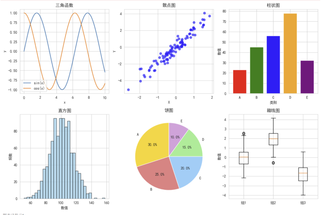
def matplotlib_basic_charts():
"""演示 Matplotlib 基础图表"""
print("=== Matplotlib 基础图表示例 ===")
# 1. 折线图
plt.figure(figsize=(12, 8))
plt.subplot(2, 3, 1)
x = np.linspace(0, 10, 100)
y1 = np.sin(x)
y2 = np.cos(x)
plt.plot(x, y1, label='sin(x)')
plt.plot(x, y2, label='cos(x)')
plt.title('三角函数')
plt.xlabel('x')
plt.ylabel('y')
plt.legend()
plt.grid(True)
# 2. 散点图
plt.subplot(2, 3, 2)
np.random.seed(42)
x = np.random.randn(100)
y = 2 * x + np.random.randn(100) * 0.5
plt.scatter(x, y, alpha=0.6, c='blue')
plt.title('散点图')
plt.xlabel('X')
plt.ylabel('Y')
# 3. 柱状图
plt.subplot(2, 3, 3)
categories = ['A', 'B', 'C', 'D', 'E']
values = [23, 45, 56, 78, 32]
plt.bar(categories, values, color=['red', 'green', 'blue', 'orange', 'purple'])
plt.title('柱状图')
plt.xlabel('类别')
plt.ylabel('数值')
# 4. 直方图
plt.subplot(2, 3, 4)
data = np.random.normal(100, 15, 1000)
plt.hist(data, bins=30, alpha=0.7, color='skyblue', edgecolor='black')
plt.title('直方图')
plt.xlabel('数值')
plt.ylabel('频数')
# 5. 饼图
plt.subplot(2, 3, 5)
sizes = [30, 25, 20, 15, 10]
labels = ['A', 'B', 'C', 'D', 'E']
colors = ['gold', 'lightcoral', 'lightskyblue', 'lightgreen', 'plum']
plt.pie(sizes, labels=labels, colors=colors, autopct='%1.1f%%', startangle=90)
plt.title('饼图')
# 6. 箱线图
plt.subplot(2, 3, 6)
data1 = np.random.normal(0, 1, 100)
data2 = np.random.normal(2, 1, 100)
data3 = np.random.normal(-2, 1, 100)
plt.boxplot([data1, data2, data3], labels=['组1', '组2', '组3'])
plt.title('箱线图')
plt.ylabel('数值')
plt.tight_layout()
plt.show()
print("图表已显示!")
# 运行示例
matplotlib_basic_charts()
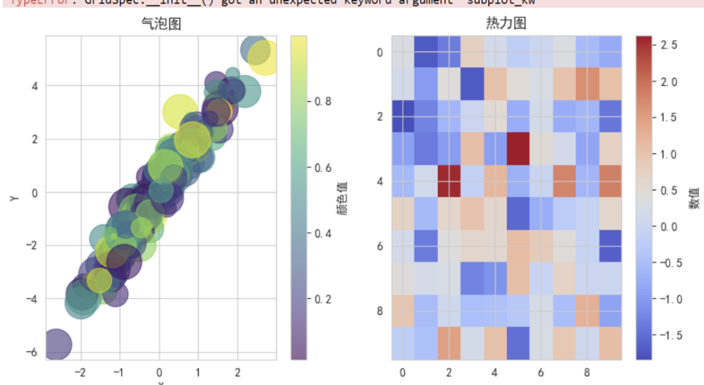
🔹高级可视化示例
# 高级可视化示例
def advanced_visualization():
    """演示高级可视化技巧"""

    print("=== 高级可视化示例 ===")

    # 创建更复杂的数据
    np.random.seed(42)
    n_points = 200

    # 生成相关数据
    x = np.random.randn(n_points)
    y = 2 * x + np.random.randn(n_points) * 0.5
    colors = np.random.rand(n_points)
    sizes = 1000 * np.random.rand(n_points)

    # 1. 气泡图
    plt.figure(figsize=(15, 5))

    plt.subplot(1, 3, 1)
    scatter = plt.scatter(x, y, c=colors, s=sizes, alpha=0.6, cmap='viridis')
    plt.colorbar(scatter, label='颜色值')
    plt.title('气泡图')
    plt.xlabel('X')
    plt.ylabel('Y')

    # 2. 热力图
    plt.subplot(1, 3, 2)
    data = np.random.randn(10, 10)
    im = plt.imshow(data, cmap='coolwarm', aspect='auto')
    plt.colorbar(im, label='数值')
    plt.title('热力图')

    # 3. 子图组合
    plt.subplot(1, 3, 3)

    # 创建子图
    gs = plt.GridSpec(2, 2, subplot_kw={'projection': 'polar'})

    ax1 = plt.subplot(gs[0, 0])
    theta = np.linspace(0, 2*np.pi, 100)
    r = np.sin(3*theta)
    ax1.plot(theta, r)
    ax1.set_title('极坐标图')

    ax2 = plt.subplot(gs[0, 1])
    categories = ['A', 'B', 'C', 'D']
    values = [15, 30, 45, 10]
    ax2.bar(categories, values)
    ax2.set_title('柱状图')

    ax3 = plt.subplot(gs[1, :])
    x_line = np.linspace(0, 10, 100)
    y_line1 = np.sin(x_line)
    y_line2 = np.cos(x_line)
    ax3.plot(x_line, y_line1, label='sin')
    ax3.plot(x_line, y_line2, label='cos')
    ax3.set_title('组合图')
    ax3.legend()

    plt.tight_layout()
    plt.show()

    print("高级图表已显示!")

# 运行示例
advanced_visualization()
Scikit-learn:机器学习的瑞士军刀🔖
什么是 Scikit-learn?
Scikit-learn 就像是机器学习的工具箱,提供了从数据预处理到模型训练、评估的完整工具链,是 Python 机器学习的事实标准。
🔹Scikit-learn 核心功能
# Scikit-learn 核心功能示例
from sklearn.datasets import make_classification, load_iris
from sklearn.model_selection import train_test_split
from sklearn.preprocessing import StandardScaler, LabelEncoder
from sklearn.linear_model import LogisticRegression
from sklearn.ensemble import RandomForestClassifier
from sklearn.svm import SVC
from sklearn.metrics import accuracy_score, classification_report, confusion_matrix

def scikit_learn_basics():
    """演示 Scikit-learn 的核心功能"""

    print("=== Scikit-learn 核心功能示例 ===")

    # 1. 数据生成
    X, y = make_classification(
        n_samples=1000,
        n_features=20,
        n_classes=3,
        n_informative=15,
        random_state=42
    )

    print(f"数据形状:X={X.shape}, y={y.shape}")
    print(f"类别分布:{np.bincount(y)}")

    # 2. 数据划分
    X_train, X_test, y_train, y_test = train_test_split(
        X, y, test_size=0.2, random_state=42, stratify=y
    )

    print(f"训练集大小:{X_train.shape[0]}")
    print(f"测试集大小:{X_test.shape[0]}")

    # 3. 数据预处理
    scaler = StandardScaler()
    X_train_scaled = scaler.fit_transform(X_train)
    X_test_scaled = scaler.transform(X_test)

    print("数据标准化完成")

    # 4. 模型训练和比较
    models = {
        '逻辑回归': LogisticRegression(random_state=42),
        '随机森林': RandomForestClassifier(n_estimators=100, random_state=42),
        '支持向量机': SVC(random_state=42)
    }

    results = {}

    for name, model in models.items():
        print(f"\n训练 {name}...")

        # 训练模型
        model.fit(X_train_scaled, y_train)

        # 预测
        y_pred = model.predict(X_test_scaled)

        # 评估
        accuracy = accuracy_score(y_test, y_pred)
        results[name] = accuracy

        print(f"{name} 准确率:{accuracy:.4f}")
        print(f"分类报告:\n{classification_report(y_test, y_pred)}")

    # 5. 结果比较
    print("\n=== 模型比较 ===")
    for name, accuracy in results.items():
        print(f"{name}: {accuracy:.4f}")

    best_model = max(results, key=results.get)
    print(f"\n最佳模型:{best_model}")

    return models[best_model]

# 运行示例
best_model = scikit_learn_basics()
=== Scikit-learn 核心功能示例 ===
数据形状:X=(1000, 20), y=(1000,)
类别分布:[329 332 339]
训练集大小:800
测试集大小:200
数据标准化完成

训练 逻辑回归...
逻辑回归 准确率:0.7200
分类报告:
              precision    recall  f1-score   support

           0       0.84      0.64      0.72        66
           1       0.67      0.74      0.71        66
           2       0.69      0.78      0.73        68

    accuracy                           0.72       200
   macro avg       0.73      0.72      0.72       200
weighted avg       0.73      0.72      0.72       200


训练 随机森林...
随机森林 准确率:0.8050
分类报告:
              precision    recall  f1-score   support

           0       0.87      0.82      0.84        66
           1       0.73      0.82      0.77        66
           2       0.83      0.78      0.80        68

    accuracy                           0.81       200
   macro avg       0.81      0.81      0.81       200
weighted avg       0.81      0.81      0.81       200


训练 支持向量机...
支持向量机 准确率:0.8450
分类报告:
              precision    recall  f1-score   support

           0       0.90      0.85      0.88        66
           1       0.78      0.88      0.83        66
           2       0.86      0.81      0.83        68

    accuracy                           0.84       200
   macro avg       0.85      0.85      0.85       200
weighted avg       0.85      0.84      0.85       200


=== 模型比较 ===
逻辑回归: 0.7200
随机森林: 0.8050
支持向量机: 0.8450

最佳模型:支持向量机
🔹完整的机器学习流程
# 完整的机器学习流程示例
def complete_ml_pipeline():
    """演示完整的机器学习流程"""

    print("=== 完整机器学习流程 ===")

    # 1. 加载数据
    iris = load_iris()
    X = iris.data
    y = iris.target
    feature_names = iris.feature_names
    target_names = iris.target_names

    print(f"数据集:{iris.DESCR.split('\n')[0]}")
    print(f"特征数量:{len(feature_names)}")
    print(f"类别数量:{len(target_names)}")

    # 2. 数据探索
    df = pd.DataFrame(X, columns=feature_names)
    df['target'] = y

    print("\n数据预览:")
    print(df.head())

    print("\n数据统计:")
    print(df.describe())

    # 3. 数据可视化
    plt.figure(figsize=(12, 4))

    plt.subplot(1, 2, 1)
    for i, target_name in enumerate(target_names):
        plt.scatter(
            df[df['target'] == i]['sepal length (cm)'],
            df[df['target'] == i]['sepal width (cm)'],
            label=target_name
        )
    plt.xlabel('花萼长度')
    plt.ylabel('花萼宽度')
    plt.title('花萼尺寸分布')
    plt.legend()

    plt.subplot(1, 2, 2)
    for i, target_name in enumerate(target_names):
        plt.scatter(
            df[df['target'] == i]['petal length (cm)'],
            df[df['target'] == i]['petal width (cm)'],
            label=target_name
        )
    plt.xlabel('花瓣长度')
    plt.ylabel('花瓣宽度')
    plt.title('花瓣尺寸分布')
    plt.legend()

    plt.tight_layout()
    plt.show()

    # 4. 数据准备
    X_train, X_test, y_train, y_test = train_test_split(
        X, y, test_size=0.3, random_state=42, stratify=y
    )

    # 5. 模型训练
    from sklearn.ensemble import RandomForestClassifier
    model = RandomForestClassifier(n_estimators=100, random_state=42)
    model.fit(X_train, y_train)

    # 6. 模型评估
    y_pred = model.predict(X_test)
    accuracy = accuracy_score(y_test, y_pred)

    print(f"\n模型准确率:{accuracy:.4f}")
    print("\n混淆矩阵:")
    print(confusion_matrix(y_test, y_pred))
    print("\n分类报告:")
    print(classification_report(y_test, y_pred, target_names=target_names))

    # 7. 特征重要性
    feature_importance = model.feature_importances_
    feature_df = pd.DataFrame({
        '特征': feature_names,
        '重要性': feature_importance
    }).sort_values('重要性', ascending=False)

    print("\n特征重要性:")
    print(feature_df)

    # 8. 特征重要性可视化
    plt.figure(figsize=(8, 4))
    plt.bar(feature_df['特征'], feature_df['重要性'])
    plt.title('特征重要性')
    plt.xlabel('特征')
    plt.ylabel('重要性')
    plt.xticks(rotation=45)
    plt.tight_layout()
    plt.show()

    return model, feature_df

# 运行示例
trained_model, feature_importance = complete_ml_pipeline()